Solving Distinct Values Queries using Mo's Algorithm (Query SQRT Decomposition) with Hilbert Curve

## SQRT Decomposition Square Root Decomposition is an technique optimizating common operations in time complexity O(sqrt(N)). The idea of this technique is to decompose the array into small blocks of size [N / sqrt(N)] = [sqrt(N)]. ```cpp b[0] : x[0], x[1], ..., x[block_size - 1] b[1] : x[block_size], ..., x[2 * block_size - 1] ... b[block_size - 1] : x[(block_size - 1) * block_size], ..., x[N - 1] ``` and precompute the answer for all blocks. Example: precalculate the sum of elements in block k. ```cpp b[k] = min(N - 1, (k + 1) * block_size - 1) Σ i = k * block_size (x[i]) ``` To calculate the sum of elements in a range [l, r], we just need the sum of [l ... (k + 1) * s - 1], [p * s ... r], and b[i]. ```cpp r Σ i = l (x[i]) = (k + 1) * block_size - 1 Σ i = l (x[i]) + p - 1 Σ i = k + 1 (b[i]) + r Σ i = p * s (x[i]) ``` ## Problem - Distinct Values Queries You are given an array of n integers and q queries of the form: how many distinct values are there in a range [a,b]? Input: ``` 5 3 3 2 3 1 2 1 3 2 4 1 5 ``` Output: ``` 2 3 3 ``` ## Solution 1 - Using Mo's Algorithm We can answer the range queries offline in O((N + Q) * sqrt(N)) using the idea based on square root decomposition. We need to answer the queries in a special order - answer all queries with L value in block 0 first, then answer all queries with L value in block 1, and so on. If they are in the same block, we then sort it by their R value. ```cpp bool operator < (const mo &m) const { // different block - sort by block if(left / block_size != m.left / block_size) return left / block_size < m.left / block_size; // same block - sort by right value return right < m.right; } ``` Then we need two functions for updating the answer - ``add`` and ``remove`` and freq[x] to keep track the frequency of a number x. For add function, if freq[x] is 0, and if we add 1 to it then x is now a distinct value. Similarly, we do it in reverse in ``remove`` function. ```cpp void add(int x) { if(!freq[x]) ans++; freq[x]++; } void remove(int x) { freq[x]--; if(!freq[x]) ans--; } ``` For each query [L, R], we can combine the precomted answer of the blocks that lie in between [L, R] in the given array. For example, given an array a[0 .. N - 1], we are asked to find out the sum in a range [L, R]. We first calculate the sum in a range [0, N - 1], if a query is like [1, N - 1], we simply substract the first element a[0] from the sum. Therefore, in general we have four cases to consider. ### Case 1: cur_left < query_left We need to substract the sum from ``cur_left`` to ``query_left``. ``` [0, 1, 2, 3, 4, 5, 6, 7, 8, 9, 10, 11, 12, 13, 14, 15, 16, 17, 18, 19, 20] ^ cur_left ^ query_left ``` ### Case 2: cur_left > query_left We need to add the sum from ``cur_left`` to ``query_left``. ``` [0, 1, 2, 3, 4, 5, 6, 7, 8, 9, 10, 11, 12, 13, 14, 15, 16, 17, 18, 19, 20] ^ query_left ^ cur_left ``` ### Case 3: cur_right < query_right We need to add the sum from ``cur_right`` to ``query_right``. ``` [0, 1, 2, 3, 4, 5, 6, 7, 8, 9, 10, 11, 12, 13, 14, 15, 16, 17, 18, 19, 20] ^ cur_right ^ query_right ``` ### Case 4: cur_right > query_right We need to substract the sum from ``query_right`` to ``cur_right``. ``` [0, 1, 2, 3, 4, 5, 6, 7, 8, 9, 10, 11, 12, 13, 14, 15, 16, 17, 18, 19, 20] ^query_right ^ cur_right ``` where - cur_left is the left pointer of the last query L - cur_right is the right pointer of the last query R - query_left is the left pointer of the query L - query_right is the right pointer of the query R ```cpp int cur_left = 0, cur_right = 0; REPN(i, q) { while(cur_left < Q[i].left) remove(x[cur_left++]); while(cur_left > Q[i].left) add(x[--cur_left]); while(cur_right < Q[i].right) add(x[++cur_right]); while(cur_right > Q[i].right) remove(x[cur_right--]); res[Q[i].idx] = ans; } ``` However, [this solution](https://cses.fi/paste/0670b45afd08a4401804dc/) only passes 3 out of 11 test cases. The verdict for the rest of them is RUNTIME ERROR.  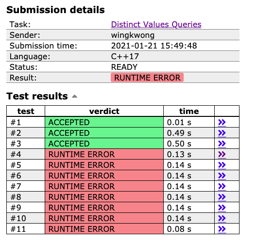The reason is that each element can go up to 10 ^ 9. We cannot use frequency array for that. We also cannot use ``unordered_map`` as it will time out due to high constant factor. Therefore, an alternative is to use coordinate compression to map the large values to smaller one in the range [1, N] as N at most can be 2 * 10 ^ 5. ```cpp int compressed = 1; map compress; REPN(i, n) { // read the input cin >> x[i]; // find the compressed value -> update x[i] if(compress.find(x[i]) != compress.end()) x[i] = compress[x[i]]; // not found -> compress it and update x[i] else compress[x[i]] = compressed, x[i] = compressed++; } ``` Now [the revised solution](https://cses.fi/paste/d8a09d857905de4a182310/) gives you 4 TIME LIMIT EXCEED verdicts.  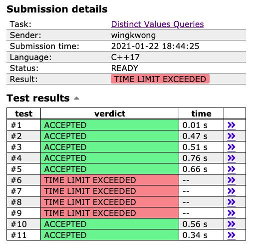Let's rethink of the time complexity. When we sort all the queries, it will take O(QlogQ). For add(x) and remove(x), let the block size be S, it takes O((N / S) * N) calls for all blocks. If S is around sqrt(N), it takes O((N + Q) * sqrt(N)) in total. The solution can be all passed by changing the block_size to 555 and even more. Therefore, we can conclude that S = sqrt(N) doesn't always give you the best runtime. Moreover, we should also use ``const`` to define the block size instead of computing it in runtime as division by constants is optimized by the compliers. Is there a way to achieve a faster sorting? Yes. We can do it in O(N * sqrt(Q)) with [Hilbert Curve](https://en.wikipedia.org/wiki/Hilbert_curve). ## Solution 2 - Using Mo's Algorithm with Hilbert Curve Hilbert Curve is a continuous fractal space-filling curve. Here's some examples. Hilbert Curve with order = 1 ``` |__| ``` Hilbert Curve with order = 2 ``` __ __ __| |__ | __ | |__| |__| ``` Hilbert Curve with order = 3 ``` __ __ __ __ |__| __| |__ |__| __ |__ __| __ | |__ __| |__ __| | |__ __ __ __ __| __| |__ __| |__ | __ | | __ | |__| |__| |__| |__| ``` For each order N > 1, it traces out a miniature order N - 1, connecting from the end of the mini curve in the lower-left to the start of the mini curve in the upper-left and from the upper-right down to the lower-right and flip the quadrant to make the connection shorter. The pattern continues like that for higher orders. If we have a point about the halfway in the frequency line in Snake Curve, the locations of the point can be different wildly as N increases. However, with Hilbert Curve, the given point moves around less and less as N increases. Therefore, we can revise our mo struct and the sorting compartor using Hilbert Order. ```cpp struct mo { int idx, left, right; int64_t ord; void set(int i, int l, int r) { idx = i, left = l, right = r, ord = hilbert_order(l, r, 21, 0); } }; inline bool operator<(const mo &a, const mo &b) { return a.ord < b.ord; } ``` Here's the implementation of Hilbert Order function. ```cpp inline int64_t hilbert_order(int x, int y, int pow, int rotate) { if (pow == 0) return 0; int hpow = 1 << (pow - 1); int seg = (x < hpow) ? ( (y < hpow) ? 0 : 3 ) : ( (y < hpow) ? 1 : 2 ); seg = (seg + rotate) & 3; const int rotate_delta[4] = {3, 0, 0, 1}; int nx = x & (x ^ hpow), ny = y & (y ^ hpow); int nrot = (rotate + rotate_delta[seg]) & 3; int64_t sub_square_size = int64_t(1) << (2 * pow - 2); int64_t ans = seg * sub_square_size, add = hilbert_order(nx, ny, pow - 1, nrot); ans += (seg == 1 || seg == 2) ? add : (sub_square_size - add - 1); return ans; } ``` We can see that [the final solution](https://cses.fi/paste/c16a9e1ae75872c6183147/) can pass all the test cases. With such technique, it works faster than the previous version, especially when N >> Q. Supposing we have a matrix with size 2 ^ k * 2 ^ k, if we divide it onto squares with size 2 ^ k - l * 2 ^ k - l, we need O(2 ^ k - l) time to travel between adjacent squares. We can process all queries in O(Q * 2 ^ k - l) = O(Q * N / sqrt(Q)) = O(N * sqrt(Q)).  At the end, it took me 74 attmepts to find out the most optimized solution.  ## Conclusion We can solve this problem using Mo's algorithm because it is an offline algorithm as we don't need to update the elements or the execution order of queries. We can utilize Hilbert Curve to speed up the program. It can also be solved using Segment Tree.

Construct Quad Tree

A quadtree is a tree data structure in which each internal node has exactly four children. Given a n * n matrix grid of 0's and 1's only. We want to represent the grid with a Quad-Tree. Return the root of the Quad-Tree representing the grid. Notice that you can assign the value of a node to True or False when isLeaf is False, and both are accepted in the answer. Definition for a QuadTree node. ```cpp class Node { public: bool val; bool isLeaf; Node* topLeft; Node* topRight; Node* bottomLeft; Node* bottomRight; Node() { val = false; isLeaf = false; topLeft = NULL; topRight = NULL; bottomLeft = NULL; bottomRight = NULL; } Node(bool _val, bool _isLeaf) { val = _val; isLeaf = _isLeaf; topLeft = NULL; topRight = NULL; bottomLeft = NULL; bottomRight = NULL; } Node(bool _val, bool _isLeaf, Node* _topLeft, Node* _topRight, Node* _bottomLeft, Node* _bottomRight) { val = _val; isLeaf = _isLeaf; topLeft = _topLeft; topRight = _topRight; bottomLeft = _bottomLeft; bottomRight = _bottomRight; } }; ``` We can construct a Quad-Tree from a two-dimensional area using the following steps: If the current grid has the same value (i.e all 1's or all 0's) set isLeaf True and set val to the value of the grid and set the four children to Null and stop. If the current grid has different values, set isLeaf to False and set val to any value and divide the current grid into four sub-grids as shown in the photo. Recurse for each of the children with the proper sub-grid. If you want to know more about the Quad-Tree, you can refer to the wiki. Quad-Tree format: The output represents the serialized format of a Quad-Tree using level order traversal, where null signifies a path terminator where no node exists below. It is very similar to the serialization of the binary tree. The only difference is that the node is represented as a list [isLeaf, val]. If the value of isLeaf or val is True we represent it as 1 in the list [isLeaf, val] and if the value of isLeaf or val is False we represent it as 0. Example: ``` Input: grid = [[0,1],[1,0]] Output: [[0,1],[1,0],[1,1],[1,1],[1,0]] ``` Solution: Recursively divide the grid by four and check if it is the leaf and its value is same as the other three. ``` Node* construct(vector>& grid) { int n = (int) grid.size(); return build(grid, 0, 0, n); } Node* build(vector>& grid, int i, int j, int n) { if(n == 1) return new Node(grid[i][j], true); Node* res = new Node(0, false, build(grid, i, j, n / 2), build(grid, i, j + n / 2, n / 2), build(grid, i + n / 2, j, n / 2), build(grid, i + n / 2, j + n / 2, n / 2)); if( res->topLeft->isLeaf && res->topRight->isLeaf && res->bottomLeft->isLeaf && res->bottomRight->isLeaf && res->topLeft->val == res->topRight->val && res->topLeft->val == res->bottomLeft->val && res->topLeft->val == res->bottomRight->val ) { res->val = res->topLeft->val; res->isLeaf = true; delete res->topLeft; delete res->topRight; delete res->bottomLeft; delete res->bottomRight; res->topLeft = NULL; res->topRight = NULL; res->bottomLeft = NULL; res->bottomRight = NULL; } return res; } ```

AtCoder - 167D. Teleporter

You can practice the problem [here](https://atcoder.jp/contests/abc167/tasks/abc167_d). ## Problem statement The Kingdom of Takahashi has N towns, numbered 1 through N. There is one teleporter in each town. The teleporter in Town i (1 <= i <= N) sends you to Town A[i]. Takahashi, the king, loves the positive integer K. The selfish king wonders what town he will be in if he starts at Town 1 and uses a teleporter exactly K times from there. Help the king by writing a program that answers this question. ## Sample Input 1 ``` 4 5 3 2 4 1 ``` ## Sample Output 1 ``` 4 ``` ## Sample Input 2 ``` 6 727202214173249351 6 5 2 5 3 2 ``` ## Sample Output 2 ``` 2 ``` ## Solution 1: Math If you take a look at the sample input 2, we can see that there is no way to traverse k times by listing out the travel. We can easily obverse the pattern the loop starts at a certain point. Example: ``` 6 5 2 5 3 2 1 -> 6 -> 2 -> 5 -> 3 -> 2 -> 5 -> 3 -> 2 -> 5 .... ``` Starting from the third step, it starts the loop 2 -> 5 -> 3. We can first create a map to store the index (0-based) and the value. ```cpp m[i] = a[i] ``` Then we can find how many steps we need to make before entering the loop, let's say ``c[i]``, and how many steps to reach the first duplicate element, let's say ``step``. ``` bool duplicate = false; ll i = 0, step = 0, kk = k; while(!duplicate && kk){ step++; // step is used to find out when a town has been visited if(d[i] == 1){ // if it is visited before, that is the start of the loop duplicate = true; continue; } d[i] = 1; // set the current i to 1, in other word, this has been visited c[i] = step; // we need to store the step to another map because we need to calculate from where the looping starts i = m[i] - 1; // -1 because it s 0 based kk--; // monitor if it s out of boundary } ``` We can calculate how many times we need to teleport from the repeating pattern as we know the length of the repeating pattern till k ``k - c[i]``, and the length of the repeating pattern ``step - c[i]``. ``` 6 5 2 5 3 2 1 -> 6 -> 2 -> 5 -> 3 -> 2 -> 5 -> 3 -> 2 -> 5 .... x x |-----------step---------| |--------------k-c[i]---------------- .... |---c[i]--| |------------------------k--------------------- .... ``` It performs only if it is not out of boundary. ```cpp if(kk){ ll r = (k - c[i]) % (step - c[i]); while(r >= 0){ i = m[i] - 1; r--; } } OUT(i + 1); ``` ## Solution 2: Binary Lifting After half a year, I came up with another solution using Binary Lifting which is a technique used to find the k-th ancestor of any node in a tree in O(logn). You can use it to find out Lowest Common Ancestor(LCA) as well. We know the ``k`` can go up to 10 ^ 18, which means we only need around 60 nodes (log2(10 ^ 18)). ```cpp const int mxN = 200005; const int mxNode = 60; // ~ log2(k) int up[mxN][mxNode]; ``` First we need to preprecess the tree in O(nlogn) using dynamic programming. ```cpp void binary_lifting() { for(int i = 1; i < mxNode; i++) { for(int u = 0; u < mxN; u++) { up[u][i] = up[up[u][i - 1]][i - 1]; } } } ``` Then we can easily find the k-th ancestor of any node in a tree in O(logn). In this case, we start from node 0. ```cpp int kth_ancestor(ll u, ll k) { for(int i = 0; i < mxNode; i++) { if(k & (1LL << i)) u = up[u][i]; } return u; } ``` The answer would be ``kth_ancestor(0, k) + 1``. ## Source Code The full solution is avilable [here](https://github.com/wingkwong/competitive-programming/blob/master/atcoder/contests/abc167/D.cpp).